Spatial Data Object

A Spatial Data Object (SDO) is the standard data output format for Teton™ CytoProfiling assays using the AVITI24™ system, designed to unify and streamline multiomics spatial data. After a cytoprofiling run, Cells2Stats converts the run output (images, cell segmentation, cell count, polony detection data) into a single structured object for downstream analysis and visualization.

An SDO is a single Zarr-based directory (RunID.zarr or .zarr.zip) containing all modalities from a run in one location and is compatible with Python-based single-cell and spatial analysis tools. The SDO format is designed to:

Provide a single entry point for all run outputs
Maintain consistent linkage between modalities
Enable direct use with existing analysis tools (e.g., Scanpy, scverse)
Reduce preprocessing and data manipulation
Enable users to quickly and efficiently access and utilize their experimental data

The SDO is a customized implementation of the SpatialData object as defined by the scverse spatialdata package and file format documentation. It conforms fully to that specification, allowing users to run analysis with any spatialdata-compatible scverse toolkit. The SDO is designed to be:

Self-contained — all run data is packaged together for maximum reproducibility and ease of sharing
Self-explainable — users familiar with scverse can naturally derive the meaning of each object by name
Structured for analysis — built-in organization simplifies querying, analyzing, and visualizing data

An SDO packages the diverse data types (imaging, transcriptomics, proteomics, morphology) from a cytoprofiling run into a single, structured object that is ready for:

Visualization using CytoCanvas™ or napari with the spatialdata plugin
Computational analysis with Python or other languages like R or Julia. The Zarr encoding is language-agnostic.
Integration with the broader single-cell ecosystem

The SDO is designed to serve as a living, run-level data repository. Users are encouraged to unzip the .zarr.zip archive and work with the Zarr store directly, enabling them to add their own processed layers of data — such as new segmentations, CellProfiler features, or additional metadata to tables.

File format and storage

Each Cells2Stats execution produces one SDO:

RunID.zarr.zip

This archive contains a hierarchical directory structure using the Zarr format, which:

Stores large datasets in chunked arrays
Supports efficient access and parallel I/O
Is compatible with local or cloud environments

Zarr characteristics

Zarr is a cloud-native, open-source file format and library for storing large, N-dimensional tensor data (arrays) efficiently. It breaks datasets into compressed, hierarchical chunks, enabling fast, parallelized read/write access ideal for scientific analysis and cloud storage.

Hierarchical (folder-like structure)
Optimized for large, multidimensional data
Follows the OME-Zarr file format specification

The SDO implements the SpatialData Zarr format, which defines the conventions for storing spatial omics data within a Zarr container.

SDO structure

The SDO structure is based on the SpatialData framework, an open and universal framework that defines how spatial omics datasets should be stored and accessed.

SDO data elements

Top-level organization:

RunID.zarr
├── images/
├── labels/
├── shapes/
├── points/
├── tables/
└── metadata/

Each directory corresponds to a specific data modality.

Mapping run output to SDO:

Run Output	SDO Component
Cell paint images	Images
Segmentation results	Labels
Transcript/protein detections	Points
Derived contours	Shapes
Cell-level measurements	Tables

The SDO does not modify the data; it reorganizes and links it within a standardized structure.

Full directory layout:

A typical targeted panel run with 12 wells and 7 batches has the following structure:

MyRun.zarr/
├── zarr.json                                # Zarr v3 store metadata
├── metadata/                                # Build provenance and input files
│
├── images/                                  # One CellPaint image stack per well
│   ├── A1-images-cell_paint/
│   ├── A2-images-cell_paint/
│   ├── B1-images-cell_paint/
│   └── ...                                  # 12 total (one per well)
│
├── labels/                                  # Cell + nuclear segmentation masks
│   ├── A1-labels-Cell/
│   ├── A1-labels-Nuclear/
│   ├── A2-labels-Cell/
│   ├── A2-labels-Nuclear/
│   └── ...                                  # 24 total (2 per well)
│
├── points/                                  # Polony locations per well × batch
│   ├── A1-points-B01/
│   ├── A1-points-B02/
│   ├── ...
│   ├── A1-points-B07/
│   └── ...                                  # wells × batches (e.g. 12 × 7 = 84)
│
├── shapes/                                  # Cell + nuclear boundary polygons
│   ├── A1-shapes-Cell/
│   ├── A1-shapes-Nuclear/
│   └── ...                                  # 24 total (2 per well)
│
└── tables/                                  # Per-cell count matrices (AnnData)
    ├── global-table-Transcript/             # RNA counts (targeted genes)
    ├── global-table-Protein/                # Protein target counts
    ├── global-table-CellPaint/              # Morphology features
    └── global-table-metadata/               # Run-level metadata (no cell data)

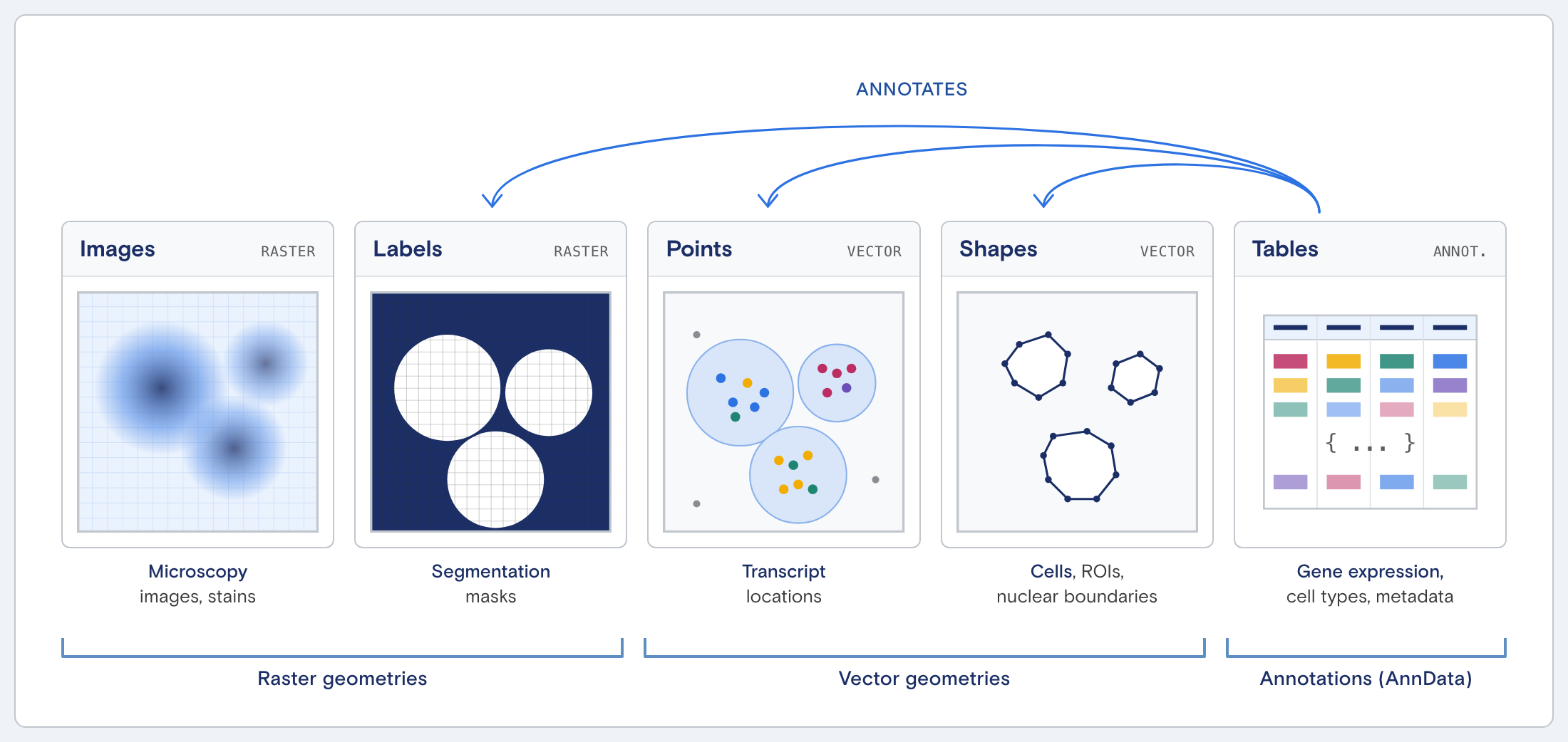
Data elements

Each SDO contains five core data elements:

Element	What it represents
Images	Multichannel fluorescent images (raster)
Labels	Segmentation masks (cell IDs, nuclei)
Points	Locations of detected molecules (RNA, protein)
Shapes	Cell/nucleus boundaries (vector contours)
Tables	Cell-level measurements (AnnData format)

Spatial vs. non-spatial elements:

Images, Labels, Points, and Shapes are spatial elements — they contain spatial coordinates or are spatial arrays. Tables are non-spatial and store cell-level measurements without inherent coordinate information. All spatial elements are connected via a coordinate system defined at the well level, which links them together within a shared spatial reference frame.

Raw and derived data:

The SDO contains both the most raw form of instrument data (images, polony point locations) and analysis-derived layers (segmentation masks, cell boundary shapes, count tables). All data is preserved in its most raw form, enabling reprocessing by users and ensuring full reproducibility.

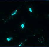
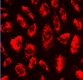
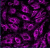
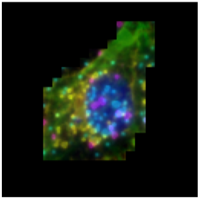
Images

Multichannel raster fluorescent images generated from cell paint assays. Depending on the run configuration, there are 3 or 6 cell paint images per well, one per channel. A 6-channel configuration includes: Nucleus, Cell Membrane, Actin, Mitochondria, Golgi, and Endoplasmic Reticulum.

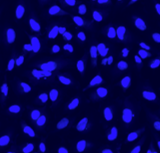
Nucleus

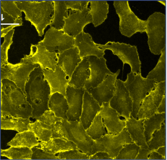
Cell Membrane

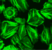
Actin

Mitochondria

Golgi

Endoplasmic
Reticulum

Images location in Spatial Data Object:

RunID.zarr/
├── images/
│   └── {well}-images-cell-paint
├── labels/
├── shapes/
├── points/
├── tables/
└── metadata/

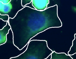
Labels

Pixel-level segmentation masks used for quantitative analysis, cell identification, and linkage.

Types:

Cell masks: integer-labeled (each cell has a unique ID)
Nuclear masks: binary (0 = background, 1 = nucleus)

Cropped image of a cell

Same cropped image with cell mask applied

Labels location in Spatial Data Object:

RunID.zarr/
├── images/
├── labels/
│   ├── {well}-labels-Cell
│   └── {well}-labels-Nuclear
├── shapes/
├── points/
├── tables/
└── metadata/

Shapes

Smoothed cell/nucleus boundaries derived from segmentation masks during SDO construction to smooth out pixel artifacts. Used for visualization (e.g., overlays in CytoCanvas).

Geometric shapes that contour the segmentation mask to smooth out pixel artifacts

Shapes location in Spatial Data Object:

RunID.zarr/
├── images/
├── labels/
├── shapes/
│   ├── {well}-shapes-Cell
│   └── {well}-shapes-Nuclear
├── points/
├── tables/
└── metadata/

Note:

Shapes are not used for quantitative measurements. Raw masks (labels) should be used for calculations.

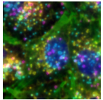
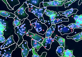
Points

Spatial (X, Y) coordinates on the image of detected molecules (transcripts or proteins), used to map molecular data back to cells. Organized by batch and well. There is a Zarr directory for every non-cell paint batch (targeted, untargeted, protein).

Point locations for transcripts and proteins

Points location in Spatial Data Object:

RunID.zarr/
├── images/
├── labels/
├── shapes/
├── points/
│   ├── {well}-points-B01
│   ├── {well}-points-B02
│   └── {well}-points-B0N ... (for N non-cell paint batches)
├── tables/
└── metadata/

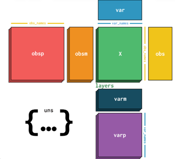
Tables (AnnData)

The Tables element uses AnnData (Annotated Data), the standard format for single-cell analysis. Tables serve as the primary linkage between the cell id and the remaining spatial data attributes.

Each table is a cell × feature matrix where rows are segmented cells and columns are measured features (genes, proteins, or morphology). There is a global-table-* (one table per modality, varies by run type) and global-table-metadata (run-level metadata, no cell data). "Global" indicates data from all wells and batches is combined into a single table.

Tables location in Spatial Data Object:

RunID.zarr/
├── images/
├── labels/
├── shapes/
├── points/
├── tables/
│   ├── global-table-metadata
│   ├── global-table-Transcript
│   ├── global-table-Protein
│   ├── global-table-CellPaint
│   ├── global-table-ThreePrimeUntargeted
│   └── global-table-{CustomBatchName}    # for OPS: global-table-{OPS Batch}-{Target Site}
└── metadata/

The tables present in the SDO depend on the assay and batches included in the run (targeted, 3', etc.). The global-table-metadata contains run-level information such as build provenance, batches, targets, wells, and tiles.

Tables are compatible with Scanpy, scverse, and Python workflows, and store both data (counts) and metadata (cell location, features, annotations).

The AnnData format of the Spatial Data Object

Different batches generate different AnnData table structures. Each table is designed to be as self-explanatory as possible. The global-table-metadata AnnData table contains thorough metadata about experimental conditions, batch types, and other run-level information.

.X: primary data matrix (raw gene counts)
.obs: cell metadata (cell ID, X/Y spatial location, area, etc.)
.var: feature metadata (information about the genes)
.obsm: cell-level matrices (geometry, QC metrics, filter flags)
.layers: additional matrices (e.g., nuclear counts)
.uns: run metadata, spatial linkage info

Modalities:

Each AVITI24 run can produce multiple modalities (assay types), depending on the panel design. Transcript and Protein are targeted modalities where the panel defines which genes/proteins are measured. CellPaint is an imaging modality where features are extracted from fluorescence images. OPS is a specialized targeted modality used in Optical Pooled Screening (OPS) experiments to assign cell identity (e.g., cell line or guide RNA).

The tables that are displayed depend on which batches were included in the cytoprofiling run.

Modality	Table Name	What it measures	Typical feature count
Transcript	`global-table-Transcript`	Assigned target counts per gene (barcoding)	100–400 genes
Protein	`global-table-Protein`	Assigned target counts per protein (barcoding)	Up to 138 proteins
Cell Paint	`global-table-CellPaint`	Cell morphology features from fluorescence imaging	500–600 features
ThreePrimeUntargeted	`global-table-ThreePrimeUntargeted`	Whole-transcriptome 3' counts (direct in-sample sequencing)	10,000+ genes
OPS	`global-table-{OPS Batch}-{Target Site}` (for example, `global-table-B01-A549`)	Optical Pooled Screening (OPS) assignments per batch and target site, where target sites are defined in the panel	Varies by screen design

Common configurations:

Configuration	Tables	Typical Batches
Targeted Panel	Transcript, Protein, CellPaint, metadata	5–7
3' Untargeted (whole transcriptome)	ThreePrimeUntargeted, CellPaint, metadata	3–5

Note:

Some tables (e.g., ThreePrimeUntargeted) are stored in sparse format to reduce memory usage for large datasets with many zero values.

Metadata

Contains SpatialData build logs, build provenance, and copies of the original instrument input files. Useful for traceability, debugging, and visualization of quality metrics upstream of SpatialData creation.

Metadata location in Spatial Data Object:

RunID.zarr/
├── images/
├── labels/
├── shapes/
├── points/
├── tables/
└── metadata/
    └── SpatialData build logs

How SDO elements link together

        Tables                           Points
┌─────────────────────┐       ┌──────────────────────────┐
│ adata.obs           │       │ points DataFrame         │
│   cell_id_global ◄──┼───────┼──► label_Cell_global     │
│   cell_id_local  ◄──┼───┐   │   x, y (pixel coords)    │
│   region_key ───────┼─┐ │   │   target_name            │
└─────────────────────┘ │ │   └──────────────────────────┘
                        │ │
        Labels          │ │        Shapes
┌─────────────────────┐ │ │   ┌──────────────────────────┐
│ A1-labels-Cell   ◄──┼─┘ └───┼──► A1-shapes-Cell        │
│   pixel value =     │       │   GeoDataFrame index =   │
│   cell_id_local     │       │   cell_id_local          │
└─────────────────────┘       └──────────────────────────┘

cell_id_global links cells across tables, points, and the entire run
cell_id_local links cells to their segmentation mask pixels and boundary polygons within a well
region_key identifies which label layer a cell belongs to (e.g., "A1-labels-Cell")

Wells, tiles, and batches

Wells

A well plate has positions labeled by row letter and column number (A1, A2, ..., F12). Each well typically contains one biological sample or condition. The WellLabel column in .obs carries the human-readable label assigned during experiment setup.

Tiles

Each well is imaged as a grid of overlapping tiles, then stitched together. A tile ID like L2R01C01S1 encodes the Lane, Row, Column, and Surface. Most analysis operates at the cell or well level; tiles are relevant mainly for spatial visualization and QC.

Batches

Batches (e.g., B01, B02, B03) group the targets that are sequenced together. Each batch is basecalled independently. Batch names appear in .var["batch_name"] and in point element keys like A1-points-B02.

Accessing SDO data

Requirements:

Python environment
spatialdata and/or anndata packages

Loading the full SDO:

import spatialdata as sd
sdata = sd.read_zarr("RunID.zarr")

Accessing tables:

gene_table = sdata.tables["global-table-Transcript"]

Loading tables directly:

import anndata as ad
gene_table = ad.read_zarr("RunID.zarr/tables/global-table-Transcript")

Note:

CytoCanvas requires a zipped SDO (.zarr.zip), but some standard Python tools require the SDO to be unzipped to use native commands. The .zarr.zip file must be extracted before using read_zarr().

Visualization with CytoCanvas

Upload workflow:

Generate SDO from Cells2Stats (1.4.0 or later)
Upload .zarr.zip file to CytoCanvas
Load dataset for visualization

Available features:

Image visualization
Segmentation overlays
Transcript/protein mapping
Cell-level inspection

Data usage:

Shapes are used for rendering boundaries
Labels and tables are used for linking and filtering data

For more information, see CytoCanvas.

Typical analysis workflows

Visualization

Inspect images and segmentation
Perform quality control
Explore spatial patterns

Table-based analysis (AnnData)

Cluster cells
Identify cell populations
Perform differential expression analysis

Spatial analysis

Map gene expression to spatial context
Analyze spatial relationships between cells
Integrate morphology and molecular data
Inspect segmentation
Explore spatial patterns
Perform QC

Notes and considerations

SDO is not a flat file; it requires compatible tools for access
Most analysis workflows rely on:
- Python (Scanpy, spatialdata)
- Visualization tools (CytoCanvas)
Tables are typically the primary entry point for analysis
Images and spatial layers are optional depending on use case

File format and storage​

Zarr characteristics​

SDO structure​

Data elements​

Images​

Labels​

Shapes​

Points​

Tables (AnnData)​

Metadata​

How SDO elements link together​

Wells, tiles, and batches​

Wells​

Tiles​

Batches​

Accessing SDO data​

Visualization with CytoCanvas​

Typical analysis workflows​

Visualization​

Table-based analysis (AnnData)​

Spatial analysis​

Notes and considerations​

External resources​

File format and storage

Zarr characteristics

SDO structure

Data elements

Images

Labels

Shapes

Points

Tables (AnnData)

Metadata

How SDO elements link together

Wells, tiles, and batches

Wells

Tiles

Batches

Accessing SDO data

Visualization with CytoCanvas

Typical analysis workflows

Visualization

Table-based analysis (AnnData)

Spatial analysis

Notes and considerations

External resources